9
Jul
July 9, 2013
Overview
In static structural analysis, it is possible to describe the operation of MSC Nastran without a detailed discussion of the fundamental equations. Due to the several types of dynamic analyses and the different mathematical form of each, some knowledge of both the physics of dynamics and the manner in which the physics is represented is important to using MSC Nastran effectively and efficiently for dynamic analysis.
You should become familiar with the notation and terminology covered in this chapter. This knowledge will be valuable to understand the meaning of the symbols and the reasons for the procedures employed in later chapters. References and Bibliography, 757 provide a list of references for structural dynamic analysis.
Dynamic Analysis Versus Static Analysis
Two basic aspects of dynamic analysis differ from static analysis. First, dynamic loads are applied as a function of time or frequency-. Second, this time or frequency-varying load application induces time or frequency-varying response (displacements, velocities, accelerations, forces, and stresses). These time or frequency-varying characteristics make dynamic analysis more complicated and more realistic than static analysis.
This chapter introduces the equations of motion for a single degree-of-freedom dynamic system (see Equations of Motion, 3), illustrates the dynamic analysis process (see Dynamic Analysis Process, 13), and characterizes the types of dynamic analyses described in this guide (see Dynamic Analysis Types, 15). Those who are familiar with these topics may want to skip to subsequent chapters.
Equations of Motion
The basic types of motion in a dynamic system are displacement u and the first and second derivatives of displacement with respect to time. These derivatives are velocity and acceleration, respectively, given below:

(1-1)
Velocity and Acceleration
Velocity is the rate of change in the displacement with respect to time. Velocity can also be described as the slope of the displacement curve. Similarly, acceleration is the rate of change of the velocity with respect to time, or the slope of the velocity curve.
Single Degree-of-Freedom System
The most simple representation of a dynamic system is a single degree-of-freedom (SDOF) system (see Figure 1-1). In an SDOF system, the time-varying displacement of the structure is defined by one component of motion u(t). Velocity u̇(t) and acceleration ü(t) are derived from the displacement.
 |
| Figure 1-1 Singe Degree-of-Freedom (SDOF) System |
Dynamic and Static Degrees-of-Freedom
Mass and damping are associated with the motion of a dynamic system. Degrees-of-freedom with mass or damping are often called dynamic degrees-of-freedom; degrees-of-freedom with stiffness are called static degrees-of-freedom. It is possible (and often desirable) in models of complex systems to have fewer dynamic degrees-of-freedom than static degrees-of-freedom.
The four basic components of a dynamic system are mass, energy dissipation (damper), resistance (spring), and applied load. As the structure moves in response to an applied load, forces are induced that are a function of both the applied load and the motion in the individual components. The equilibrium equation representing the dynamic motion of the system is known as the equation of motion.
Equation of Motion
This equation, which defines the equilibrium condition of the system at each point in time, is represented as

(1-2)
The equation of motion accounts for the forces acting on the structure at each instant in time. Typically, these forces are separated into internal forces and external forces. Internal forces are found on the left-hand side of the equation, and external forces are specified on the right-hand side. The resulting equation is a second-order linear differential equation representing the motion of the system as a function of displacement and higher-order derivatives of the displacement.
Inertia Force
An accelerated mass induces a force that is proportional to the mass and the acceleration. This force is called the inertia force mü(t).
Viscous Damping
The energy dissipation mechanism induces a force that is a function of a dissipation constant and the velocity. This force is known as the viscous damping force bu̇(t). The damping force transforms the kinetic energy into another form of energy, typically heat, which tends to reduce the vibration.
Elastic Force
The final induced force in the dynamic system is due to the elastic resistance in the system and is a function of the displacement and stiffness of the system. This force is called the elastic force or occasionally the spring force ku(t).
Applied Load
The applied load p(t) on the right-hand side of Eq. (1-2) is defined as a function of time. This load is independent of the structure to which it is applied (e.g., an earthquake is the same earthquake whether it is applied to a house, office building, or bridge), yet its effect on different structures can be very different.
Solution of the Equation of Motion
The solution of the equation of motion for quantities such as displacements, velocities, accelerations, and/or stresses—all as a function of time—is the objective of a dynamic analysis. The primary task for the dynamic analyst is to determine the type of analysis to be performed. The nature of the dynamic analysis in many cases governs the choice of the appropriate mathematical approach. The extent of the information required from a dynamic analysis also dictates the necessary solution approach and steps.
Dynamic analysis can be divided into two basic classifications: free vibrations and forced vibrations. Free vibration analysis is used to determine the basic dynamic characteristics of the system with the right-hand side of Eq. (1-2) set to zero (i.e., no applied load). If damping is neglected, the solution is known as undamped free vibration analysis.
Free Vibration Analysis
In undamped free vibration analysis, the SDOF equation of motion reduces to

(1-3)
Eq. (1-3) has solution of the form

(1-4)
The quantity u(t) is the solution for the displacement as a function of time t. As shown in Eq. (1-4), the response is cyclic in nature.
Circular Natural Frequency
One property of the system is termed the circular natural frequency of the structure ωn. The subscript n indicates the “natural” for the SDOF system. In systems having more than one mass degree of freedom and more than one natural frequency, the subscript may indicate a frequency number. For an SDOF system, the circular natural frequency is given by

(1-5)
The circular natural frequency is specified in units of radians per unit time.
Natural Frequency
The natural frequency fn is defined by

(1-6)
The natural frequency is often specified in terms of cycles per unit time, commonly cycles per second (cps), which is more commonly known as Hertz (Hz). This characteristic indicates the number of sine or cosine response waves that occur in a given time period (typically one second).
The reciprocal of the natural frequency is termed the period of response Tn given by

(1-7)
The period of the response defines the length of time needed to complete one full cycle of response.
In the solution of Eq. (1-4), A and B are the integration constants. These constants are determined by considering the initial conditions in the system. Since the initial displacement of the system u(t = 0) and the initial velocity of the system u̇(t = 0) are known, A and B are evaluated by substituting their values into the solution of the equation for displacement and its first derivative (velocity), resulting in
(1-8)
These initial value constants are substituted into the solution, resulting in

(1-9)
Eq. (1-9) is the solution for the free vibration of an undamped SDOF system as a function of its initial displacement and velocity. Graphically, the response of an undamped SDOF system is a sinusoidal wave whose position in time is determined by its initial displacement and velocity as shown in Figure 1-2.
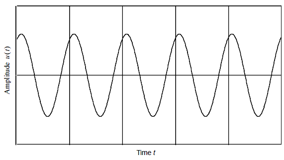 |
| Figure 1-2 SDOF System – Undamped Free Vibrations |
If damping is included, the damped free vibration problem is solved. If viscous damping is assumed, the equation of motion becomes

(1-10)
Damping Types
The solution form in this case is more involved because the amount of damping determines the form of the solution. The three possible cases for positive values of b are
- Critically damped
- Overdamped
- Underdamped
Critical damping occurs when the value of damping is equal to a term called critical damping bcr. The critical damping is defined as

(1-11)
For the critically damped case, the solution becomes

(1-12)
Under this condition, the system returns to rest following an exponential decay curve with no oscillation. A system is overdamped when b > bcr and no oscillatory motion occurs as the structure returns to its undisplaced position.
The most common damping case is the underdamped case where b < bcr. In this case, the solution has the form

(1-13)
Again, A and B are the constants of integration based on the initial conditions of the system. The new term ωd represents the damped circular natural frequency of the system. This term is related to the undamped circular natural frequency by the following expression:

(1-14)
The term ζ is called the damping ratio and is defined by

(1-15)
The damping ratio is commonly used to specify the amount of damping as a percentage of the critical damping.
In the underdamped case, the amplitude of the vibration reduces from one cycle to the next following an exponentially decaying envelope. This behavior is shown in Figure 1-3. The amplitude change from one cycle to the next is a direct function of the damping. Vibration is more quickly dissipated in systems with more damping.
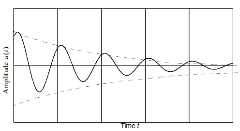 |
| Figure 1-3 Damped Oscillation, Free Vibration |
The damping discussion may indicate that all structures with damping require damped free vibration analysis. In fact, most structures have critical damping values in the 0 to 10% range, with values of 1 to 5% as the typical range. If you assume 10% critical damping, Eq. (1-4) indicates that the damped and undamped natural frequencies are nearly identical. This result is significant because it avoids the computation of damped natural frequencies, which can involve a considerable computational effort for most practical problems. Therefore, solutions for undamped natural frequencies are most commonly used to determine the dynamic characteristics of the system (see Real Eigenvalue Analysis, 43). However, this does not imply that damping is neglected in dynamic response analysis. Damping can be included in other phases of the analysis as presented later for frequency and transient response (see Frequency Response Analysis, 133 and Transient Response Analysis, 201).
Forced Vibration Analysis
Forced vibration analysis considers the effect of an applied load on the response of the system. Forced vibrations analyses can be damped or undamped. Since most structures exhibit damping, damped forced vibration problems are the most common analysis types.
The type of dynamic loading determines the mathematical solution approach. From a numerical viewpoint, the simplest loading is simple harmonic (sinusoidal) loading. In the undamped form, the equation of motion becomes

(1-16)
In this equation the circular frequency of the applied loading is denoted by ω. This loading frequency is entirely independent of the structural natural frequency ωn, although similar notation is used.
This equation of motion is solved to obtain


(1-17)
Again, A and B are the constants of integration based on the initial conditions. The third term in
Eq. (1-17) is the steady-state solution. This portion of the solution is a function of the applied loading and the ratio of the frequency of the applied loading to the natural frequency of the structure.
The numerator and denominator of the third term demonstrate the importance of the relationship of the structural characteristics to the response. The numerator p/k is the static displacement of the system. In other words, if the amplitude of the sinusoidal loading is applied as a static load, the resulting static displacement u is p/k . In addition, to obtain the steady state solution, the static displacement is scaled by the denominator.
The denominator of the steady-state solution contains the ratio between the applied loading frequency and the natural frequency of the structure.
Dynamic Amplification Factor for No Damping
The term
 Factor")
(1-18)
is called the dynamic amplification (load) factor. This term scales the static response to create an amplitude for the steady state component of response. The response occurs at the same frequency as the loading and in phase with the load (i.e., the peak displacement occurs at the time of peak loading). As the applied loading frequency becomes approximately equal to the structural natural frequency, the ratio ω/ωn approaches unity and the denominator goes to zero. Numerically, this condition results in an infinite (or undefined) dynamic amplification factor. Physically, as this condition is reached, the dynamic response is strongly amplified relative to the static response. This condition is known as resonance. The resonant buildup of response is shown in Figure 1-4.
 |
| Figure 1-4 Harmonic Forced Response with No Damping |
It is important to remember that resonant response is a function of the natural frequency and the loading frequency. Resonant response can damage and even destroy structures. The dynamic analyst is typically assigned the responsibility to ensure that a resonance condition is controlled or does not occur.
Solving the same basic harmonically loaded system with damping makes the numerical solution more complicated but limits resonant behavior. With damping, the equation of motion becomes

(1-19)
In this case, the effect of the initial conditions decays rapidly and may be ignored in the solution. The solution for the steady-state response is

(1-20)
The numerator of the above solution contains a term that represents the phasing of the displacement response with respect to the applied loading. In the presence of damping, the peak loading and peak response do not occur at the same time. Instead, the loading and response are separated by an interval of time measured in terms of a phase angle θ as shown below:

(1-21)
The phase angle θ is called the phase lead, which describes the amount that the response leads the applied force.
Note: Some texts define θ as the phase lag, or the amount that the response lags the applied force. To convert from phase lag to phase lead, change the sign of in Eq. (1-20) and Eq. (1-21).
Dynamic Amplification Factor with Damping
The dynamic amplification factor for the damped case is

(1-22)
The interrelationship among the natural frequency, the applied load frequency, and the phase angle can be used to identify important dynamic characteristics. If ω/ωn is much less than 1, the dynamic amplification factor approaches 1 and a static solution is represented with the displacement response in phase with the loading. If ω/ωn is much greater than 1, the dynamic amplification factor approaches zero, yielding very little displacement response. In this case, the structure does not respond to the loading because the loading is changing too fast for the structure to respond. In addition, any measurable displacement response will be 180 degrees out of phase with the loading (i.e., the displacement response will have the opposite sign from the force). Finally if ω/ωn = 1 , resonance occurs. In this case, the magnification factor is 1/(2ζ), and the phase angle is 270 degrees. The dynamic amplification factor and phase lead are shown in Figure 1-5 and are plotted as functions of forcing frequency.
 |
| Figure 1-5 Harmonic Forced Response with Damping |
In contrast to harmonic loadings, the more general forms of loading (impulses and general transient loading) require a numerical approach to solving the equations of motion. This technique, known as numerical integration, is applied to dynamic solutions either with or without damping. Numerical integration is described in Transient Response Analysis, 201.
Dynamic Analysis Process
Before conducting a dynamic analysis, it is important to define the goal of the analysis prior to the formulation of the finite element model. Consider the dynamic analysis process to be represented by the steps in Figure 1-6. The analyst must evaluate the finite element model in terms of the type of dynamic loading to be applied to the structure. This dynamic load is known as the dynamic environment. The dynamic environment governs the solution approach (i.e., normal modes, transient response, frequency response, etc.). This environment also indicates the dominant behavior that must be included in the analysis (i.e., contact, large displacements, etc.). Proper assessment of the dynamic environment leads to the creation of a more refined finite element model and more meaningful results.
 |
| Figure 1-6 Overview of Dynamic Analysis Process |
An overall system design is formulated by considering the dynamic environment. As part of the evaluation process, a finite element model is created. This model should take into account the characteristics of the system design; and just as importantly, the nature of the dynamic loading (type and frequency); and any interacting media (fluids, adjacent structures, etc.). At this point, the first step in many dynamic analyses is a modal analysis to determine the structure’s natural frequencies and mode shapes (see Real Eigenvalue Analysis, 43).
In many cases the natural frequencies and mode shapes of a structure provide enough information to make design decisions. For example, in designing the supporting structure for a rotating fan, the design requirements may require that the natural frequency of the supporting structure have a natural frequency either less than 85% or greater than 110% of the operating speed of the fan. Specific knowledge of quantities such as displacements and stresses are not required to evaluate the design.
Forced response is the next step in the dynamic evaluation process. The solution process reflects the nature of the applied dynamic loading. A structure can be subjected to a number of different dynamic loads with each dictating a particular solution approach. The results of a forced-response analysis are evaluated in terms of the system design. Necessary modifications are made to the system design. These changes are then applied to the model and analysis parameters to perform another iteration on the design. The process is repeated until an acceptable design is determined, which completes the design process.
The primary steps in performing a dynamic analysis are summarized as follows:
- Define the dynamic environment (loading).
- Formulate the proper finite element model.
- Select and apply the appropriate analysis approach(es) to determine the behavior of the structure.
- Evaluate the results.
Dynamic Analysis Types
This guide describes the types of dynamic analysis that can be performed with MSC Nastran. The basic types are:
- Real eigenvalue analysis (undamped free vibrations).
- Linear frequency response analysis (steady-state response of linear structures to loads that vary as a function of frequency).
- Linear transient response analysis (response of linear structures to loads that vary as a function of time).
Real eigenvalue analysis is used to determine the basic dynamic characteristics of a structure. The results of an eigenvalue analysis indicate the frequencies and shapes at which a structure naturally tends to vibrate. Although the results of an eigenvalue analysis are not based on a specific loading, they can be used to predict the effects of applying various dynamic loads. Real eigenvalue analysis is described in Real Eigenvalue Analysis, 43.
Frequency response analysis is an efficient method for finding the steady-state response to sinusoidal excitation. In frequency response analysis, the loading is a sine wave for which the frequency, amplitude, and phase are specified. Frequency response analysis is limited to linear elastic structures. Frequency response analysis is described in Frequency Response Analysis, 133.
Transient response analysis is the most general method of computing the response to time-varying loads. The loading in a transient analysis can be of an arbitrary nature, but is explicitly defined (i.e., known) at every point in time. The time-varying (transient) loading can also include nonlinear effects that are a function of displacement or velocity. Transient response analysis is most commonly applied to structures with linear elastic behavior. Transient response analysis is described in Transient Response Analysis, 201.
Additional MSC Nastran advanced dynamic analysis capabilities, such as damping, direct enforced motion, random response analysis, response spectrum analysis and coupled fluid structure analysis can be used in conjunction with the above analyses. More advanced dynamic analysis capabilities like design sensitivity, design optimization, aeroelastic, rotor dynamics, control system and nonlinear transient also build on these capabilities.
In practice, very few engineers use all of the dynamic analysis types in their work. Therefore, it may not be important for you to become familiar with all of the types. Each type can be considered independently, although there may be many aspects common to many of the analyses.
The majority of this content was directly cited from page 1 of the MSC Nastran 2012 Dynamic Analysis User's Guide.
Relevant engineering software: MSC Nastran for FEA.


Comments
C S BHATTACHARYA
Good effective explanation,
would be thankful to have more insight on this topic
regards,
thanks
c s bhattacharya