The mesh density in a finite element model is an important topic because of its relationship to accuracy and cost. In many instances, the minimum number of elements is set by topological considerations, for example, one element per member in a space frame or one element per panel in a stiffened shell structure. In the past, when problem size was more severely limited, it was not uncommon to lump two or more frames or other similar elements in order to reduce the size of the model. With computers becoming faster and cheaper, the current trend is to represent all major components individually in the finite element model.
If the minimum topological requirements are easily satisfied, the question remains as to how fine to subdivide the major components. The question is particularly relevant for elastic continua, such as slabs and unreinforced shells. In general, as the mesh density increases, you can expect the results to become more accurate. The mesh density required can be a function of many factors. Among them are the stress gradients, the type of loadings, the boundary conditions, the element types used, the element shapes, and the degree of accuracy desired.
The grid point spacing should typically be the smallest in regions where stress gradients are expected to be the steepest. Figure 9-7 shows a typical example of a stress concentration near a circular hole. The model is a circular disk with an inner radius = a and an outer radius = b. A pressure load pi is applied to the inner surface. Due to symmetry, only half of the disk is modeled. In the example, both the radial stress and the circumferential stress decrease as a function of l / r2 from the center of the hole. The error in the finite element analysis arises from differences between the real stress distribution and the stress distribution within the finite elements.
In a study of mesh densities, elements and output options, three different mesh densities were used in the example as shown in Figure 9-7. The first one is a coarse mesh model with the elements evenly distributed. The second model consists of the same number of elements; however, the mesh is biased toward the center of the hole. The third model consists of a denser mesh with the elements evenly distributed. These three models are then analyzed with three different element types-CQUAD4, CQUAD8, and CQUAD4 with the corner stress option. The circumferential stress at the inner radius is always greater than pi , which is the applied pressure load at the inner radius, and approaches this value as the outer radius becomes larger. The theoretical circumferential stress sq (see Timoshenko and Goodier, Theory of Elasticity, Reference 3.) is given by the following equation:

where:
a = inner radius
b = outer radius
r = radial distance as measured from the center of the disk
pi = pressure applied at the inner radius
The stresses are then plotted as a function of the radius in a nondimensional fashion-stress pi versus
r / a. The results are summarized in Table 9-1.
 |
| Figure 9-7 Circular Disk with Different Meshes |
Table 9-1 Stresses Close to r = a for a Circular Disk
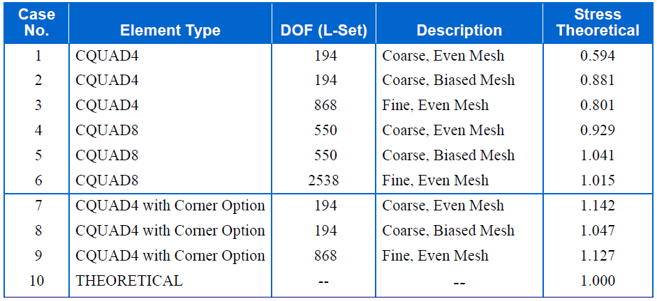
For this particular case, since the stresses are proportional to l / r2, you expect the highest stress to occur at the inner radius. In order to take advantage of this piece of information, the obvious thing to do is to create a finer mesh around the inner radius. Looking at the results for the first two cases in Table 9-1, it is quite obvious that just by biasing the mesh, the results are 30% closer to the theoretical solution with the same number of degrees of freedom.
A third case is analyzed with a finer but unbiased mesh. It is interesting to note that for case number 3, even though it has more degrees of freedom, the result is still not as good as that of case number 2. This poor result is due to the fact that for the CQUAD4 element, the stresses, by default, are calculated at the center of the element and are assumed to be constant throughout the element. Looking at Figure 9-7, it is also obvious that the centers of the inner row of elements are actually further away from the center of the circle for case number 3 as compared to case number 2. The results for case number 3 can, of course, be improved drastically by biasing the mesh.
You can request corner outputs (stress, strain, and force) for CQUAD4 in addition to the center values (Shell Elements (CTRIA3, CTRIA6, CTRIAR, CQUAD4, CQUAD8, CQUADR) (Ch. 1) in the MSC Nastran Reference Manual). Corner results are extrapolated from the corner displacements and rotations by using a strain rosette analogy with a cubic correction for bending. The same three models are then rerun with this corner option–their results are summarized in cases 7 through 9. Note that the results can improve substantially for the same number degrees of freedom.
Corner output is selected by using a corner output option with the STRESS, STRAIN, and FORCE Case Control commands. When one of these options is selected, output is computed at the center and four corners for each CQUAD4 element, in a format similar to that of CQUAD8 and CQUADR elements. See Reference 8. for more information.
There are four corner output options available: CORNER, CUBIC, SGAGE, and BILIN. The different options provide for different approaches to the stress calculations. The default option is CORNER, which is equivalent to BILIN. BILIN has been shown to produce better results for a wider range of problems.
To carry it a step further, the same three models are then rerun with CQUAD8 (cases 4 through 6). In this case, the results using CQUAD8 are better than those using the CQUAD4. This result is expected since CQUAD8 contains more DOFs per element than CQUAD4. Looking at column three of Table 9-1, you can see that due to the existence of midside nodes, the models using CQUAD8 contain several times the number of DOFs as compared to CQUAD4 for the same number of elements. The results using CQUAD4 can, of course, be improved by increasing the mesh density to approach that of the CQUAD8 in terms of number of DOFs.
It is important to realize that the stresses are compared at different locations for Cases 1 through 3 versus Cases 4 through 9. This difference occurs because the stresses are available only at the element centers for Cases 1 through 3, but the stresses are available at the corners as well as the element centers for Cases 4 through 9. When looking at your results using a stress contour plot, you should be aware of where the stresses are being evaluated.
How fine a mesh you want depends on many factors. Among them is the cost you are willing to pay versus the accuracy you are receiving. The cost increases with the number of DOFs. The definition of cost has changed with time. In the past, cost is generally associated with computer time. With both hardware and software becoming faster each day, cost is probably associated more with the time required for you to debug and interpret your results. In general, the larger the model is, the more time it takes you to debug and interpret your results. As for acceptable accuracy, proceeding from case 8 to case 6, the error is reduced from 4.7% to 1.5%; however, the size of the problem is also increased from 194 to 2538 DOFs. In some cases, a 4.7% error may be acceptable. For example, in cases in which you are certain of the loads to within only a 10% accuracy, a 4.7% error may be acceptable. In other cases, a 1.5% error may not be acceptable.
In general, if you can visualize the form of the solution beforehand, you can then bias the grid point distribution. However, this type of information is not necessarily available in all cases. If a better assessment of accuracy is required and resources are available (time and money), you can always establish error bounds for a particular problem by constructing and analyzing multiple mesh spacings of the same model and observe the convergences. This approach, however, may not be realistic due to the time constraint.
The stress discontinuity feature, as described in Model Verification (Ch. 10), may be used for accessing the quality of the mesh density for the conventional h-version elements.
Getting a good starting mesh density can be very useful, but there are mesh refinements which can be performed “automatically” inside MSC Nastran. One is the use of Local Adaptive Mesh Refinement (Ch. 18) for h-elements. The other is the use of p-version elements and p-version adaptivity. Discussion of the p-version element is beyond the scope of this user’s guide. However a basic definition of the h- version and p-version elements is warranted.
h-elements
In traditional finite element analysis, as the number of elements increases, the accuracy of the solution improves. The accuracy of the problem can be measured quantitatively with various entities, such as strain energies, displacements, and stresses, as well as in various error estimation methods, such as simple mathematical norm or root-mean-square methods. The goal is to perform an accurate prediction on the behavior of your actual model by using these error analysis methods. You can modify a series of finite element analyses either manually or automatically by reducing the size and increasing the number of elements, which is the usual h-adaptivity method. Each element is formulated mathematically with a certain predetermined order of shape functions. This polynomial order does not change in the h- adaptivity method. The elements associated with this type of capability are called the h-elements.
p-elements
A different method used to modify the subsequent finite element analyses on the same problem is to increase the polynomial order in each element while maintaining the original finite element size and mesh. The increase of the interpolation order is internal, and the solution stops automatically once a specified error tolerance is satisfied. This method is known as the p-adaptivity method. The elements associated with this capability are called the p-elements. For more details on the subject of the p-version element, refer to p-Elements (p. 194) in the MSC Nastran Reference Manual.
Mesh transition can also be made with CINTC elements for connecting meshes on dissimilar edges. Linear contact methods may also be used.
All of the content in this blog post has been directly extracted from Chapter 9 of the MSC Nastran 2012 Linear Static Analysis User's Guide.


Leave A Reply